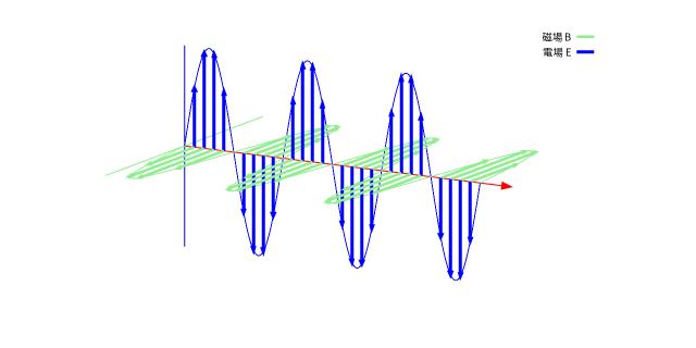
$x$ 方向に進む平面電磁波の例
真空中のマクスウェル方程式
\begin{eqnarray}
\nabla\cdot \boldsymbol{E} &=& 0 \tag{1}\\
\nabla\cdot\boldsymbol{B} &=& 0 \tag{2}\\
\nabla\times\boldsymbol{E} + \frac{\partial \boldsymbol{B}}{\partial t} &=& \boldsymbol{0} \tag{3}\\
\frac{1}{\mu_0}\nabla\times\boldsymbol{B} –
\varepsilon_0\frac{\partial \boldsymbol{E}}{\partial t} &=& \boldsymbol{0} \tag{4}
\end{eqnarray}
電場ベクトル
まず,$x$ 方向の平面電磁波(電場)がみたすべき波動方程式
$$\frac{\partial^2 \boldsymbol{E}}{\partial x^2} – \frac{1}{c^2} \frac{\partial^2 \boldsymbol{E}}{\partial t^2} = \boldsymbol{0}$$
の解として
$$\boldsymbol{E} = \boldsymbol{E}_0\,\cos(x – c t)$$
を考える。
$(1)$ 式 $\displaystyle \nabla\cdot\boldsymbol{E} = \frac{\partial E_x}{\partial x} = 0$ より $E_x = 0$ である。ここでは,$\boldsymbol{E}_0 \Rightarrow (0, 0, E_0)$ とおこう。
$$\therefore\ \ \boldsymbol{E} = \left(0, 0, E_0 \cos(x – c t) \right)$$
磁場ベクトル
次に,磁場 $\boldsymbol{B}$ も同じ波動方程式をみたすことから
$$\boldsymbol{B} = \boldsymbol{B}_0\,f(x – c t)$$
とおける。
$(2)$ 式 $\displaystyle \nabla\cdot\boldsymbol{B} = \frac{\partial B_x}{\partial x} = 0$ より $B_x = 0$ である。
また,$(3)$ 式の $z$ 成分は
$$\frac{\partial B_z}{\partial t} =
– \left(\frac{\partial E_y}{\partial x}- \frac{\partial E_x}{\partial y}\right) = 0$$
であるから,$B_z = 0$ である。
また,$(3)$ 式の $y$ 成分は
$$\frac{\partial B_y}{\partial t} =
– \left(\frac{\partial E_z}{\partial x}- \frac{\partial E_x}{\partial z}\right)$$
これから $B_y$ が以下のように得られる。
$$\therefore\ \ \boldsymbol{B} = \left(0, B_0 \cos(x – c t), 0 \right)= \left(0, -\frac{E_0}{c} \cos(x – c t), 0 \right)$$
適宜,定数部分を規格化して
\begin{eqnarray}
\boldsymbol{E} &=& \left(0, 0, E_0 \cos(x – c t) \right) \Rightarrow (0, 0, \cos(x-t))\\
\boldsymbol{B} &=& \left(0, -\frac{E_0}{c} \cos(x – c t), 0 \right)\Rightarrow (0, -\cos(x-t), 0)
\end{eqnarray}
reset
# 電磁場
Ez(x, t) = cos(x - t)
By(x, t) = - cos(x - t)
E(x, t) = abs(Ez(x, t))
B(x, t) = abs(By(x, t))
# 三項演算子を用いた条件分岐を使って
# 最背面のベクトルから描くための定義
# 後ろになって隠れるベクトルを先に描く
Ezp(x, t) = (Ez(x, t)>0) ? Ez(x, t):0
Ezm(x, t) = (Ez(x, t)<0) ? Ez(x, t):0
Byp(x, t) = (By(x, t)>0) ? By(x, t):0
Bym(x, t) = (By(x, t)<0) ? By(x, t):0

reset
unset xtics
unset ytics
unset ztics
unset border
#set zeroaxis

xini = -pi/2
xend = 6.*pi-pi/2
N = 30
dx = (xend-xini)/N

# ベクトルの始点の座標データファイル作成
set print "on-x-axis.txt"
do for [i=0: N] {
  x = xini + dx * i
  print sprintf("%8.4f  %8.4f  %8.4f", x, 0, 0)
  }
set print

set xrange [xini:xend+2]
set yrange [-1.2:1.2]
set zrange [-1.2:1.2]
set view ,,,1.7
set samples 1000, 1000
set parametric
set key inside sample 2
set arrow 1 from xini,0,0 to xend+2,0,0 lw 2 lc "red" lt 3 filled head size graph 0.02,20
set arrow 2 from xini,0,-1 to xini,0,1 lw 2 lc "blue" lt 3 filled nohead
set arrow 3 from xini,-1,0 to xini,1,0 lw 2 lc "light-green" lt 3 filled nohead

T=0
splot [x=xini:xend] \
      x, 0, Ez(x,T) lc "blue" notitle, \
      x, By(x,T), 0 lc "light-green" notitle, \
      "on-x-axis.txt" using 1:2:3:(0):(Byp($1, T)):(0) w vec \
      lw 5 lc "light-green" filled size graph 0.005,20 head title "磁場 B", \
      "" using 1:2:3:(0):(0):(Ezp($1, T)) w vec \
      lw 6 lc "blue" filled size graph 0.005,20 head title "電場 E", \
      "" using 1:2:3:(0):(0):(Ezm($1, T)) w vec \
      lw 6 lc "blue" filled size graph 0.005,20 head notitle, \
      "" using 1:2:3:(0):(Bym($1, T)):(0) w vec \
      lw 5 lc "light-green" filled size graph 0.005,20 head notitle
# terminal を pngcairo (png) に
set terminal pngcairo size 1280,640 font 'Noto Sans CJK JP,14'

# ファイル名を連番にして T を変えながら replot して保存
do for [j=1:2*N]{
  set output sprintf("%03d.png", j)
    T = dx/2*j
    replot
  set output
}
# ffmpeg で 連番 png 画像ファイルを mp4 に
! rm -f out.mp4
! ffmpeg -hide_banner -loglevel error -stream_loop 2 -framerate 10 -i %03d.png -vcodec libx264 -pix_fmt yuv420p out.mp4