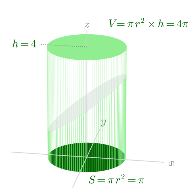
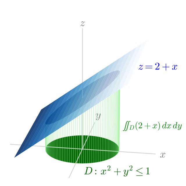
累次積分の例題の説明で使っているので。斜め切りの立体は側面をうまく描くことがわからなくて,とりあえずは,なんちゃって立体,みたいに縦線で表してみる。
必要なモジュールの import と設定
In [1]:
import matplotlib.pyplot as plt
import numpy as np

# グラフを SVG で Notebook にインライン表示
%config InlineBackend.figure_formats = ['svg']

plt.rcParams['mathtext.fontset'] = 'cm'
円柱
In [2]:
def zconst(z):
    return z*np.outer(np.ones(Ndiv), np.ones(Ndiv))
In [3]:
fig = plt.figure(figsize=[6.4, 6.4])
ax = fig.add_subplot(projection='3d')
fig.subplots_adjust(bottom=0,left=0)

# 底面
Ndiv = 180
rho = np.linspace(0, 1, Ndiv)
phi = np.linspace(0, 2*np.pi, Ndiv)
x = np.outer(rho, np.cos(phi))
y = np.outer(rho, np.sin(phi))
ax.plot_surface(x, y, zconst(0),
                color="lightgreen",
                zorder=0)

# 側面
X = np.outer(1*np.ones(Ndiv), np.cos(phi))
Y = np.outer(1*np.ones(Ndiv), np.sin(phi))
z = np.linspace(0, 4, Ndiv)
Z = np.outer(z, np.ones(Ndiv))
ax.plot_surface(X, Y, Z,
                color="lightgreen",
                alpha=0.8, zorder=10)
# 上底面
ax.plot_surface(x, y, zconst(4),
                color="lightgreen",
                zorder=20)

ax.set_xlim(-2.5, 2.5)
ax.set_ylim(-2.5, 2.5)
ax.set_zlim(0, 5)

ax.view_init(elev = 20, azim = -80, roll = 0)
ax.axis(False);
# svg ファイルは巨大になる。
# plt.savefig("enchu00.svg");
plt.savefig("Enchu00.png", dpi=360);

In [4]:
def f(x, y):
    return 2 + x
In [5]:
fig = plt.figure(figsize=[6.4, 6.4])
ax = fig.add_subplot(projection='3d')
fig.subplots_adjust(bottom=-0.1,left=0)
# 領域 D
Ndiv = 60
rho = np.linspace(0, 1, Ndiv)
phi = np.linspace(0, 2*np.pi, Ndiv)
x = np.outer(rho, np.cos(phi))
y = np.outer(rho, np.sin(phi))
ax.plot_surface(x, y, zconst(0), fc="darkgreen", ec="darkgreen",
lw = 0.2, zorder=0)
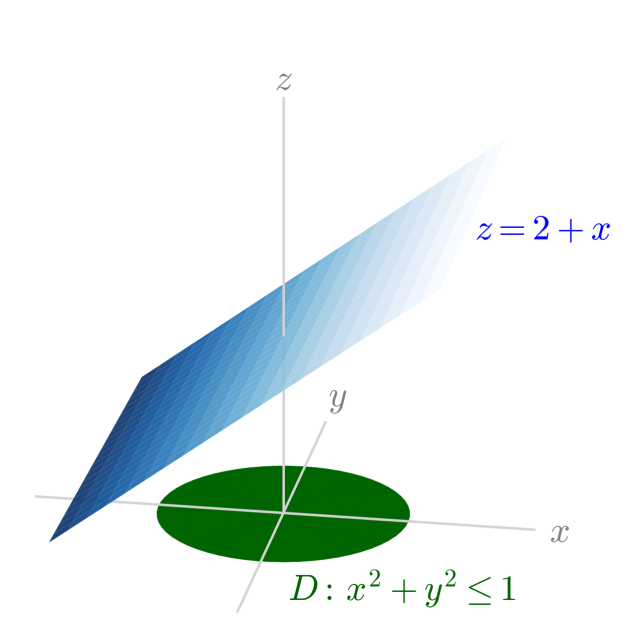
ax.text(0.3, -1.5, 0,
"$D: \, x^2 + y^2 \leq 1$", c='darkgreen',
fontsize="x-large", va="center")
# x 軸
plt.plot([-2,2], [0,0], [0,0],
lw = 1, c = "lightgray", zorder=3)
ax.text(2.2, 0, 0, "$x$",
fontsize="x-large", ha="center", va="center", c='gray')
# y 軸
plt.plot([0,0], [-2,2], [0,0],
lw = 1, c = "lightgray", zorder=3)
ax.text(0, 2.6, 0, "$y$",
fontsize="x-large", ha="center", va="center", c='gray')
# z 軸
plt.plot([0,0], [0,0], [0,2], lw = 1, c = "lightgray", zorder=3)
plt.plot([0,0], [0,0], [2,4], lw = 1, c = "lightgray", zorder=4)
plt.plot([0,0], [0,0], [4,4.6], lw = 1, c = "lightgray", zorder=10)
ax.text(0, 0, 4.8, "$z$",
fontsize="x-large", ha="center", va="center", c='gray')
# z = f(x, y)
x = np.linspace(-1.5, 1.5, 21)
y = np.linspace(-1.8, 1.8, 21)
x, y = np.meshgrid(x, y)
ax.plot_surface(x, y, f(x, y),
cmap = "Blues_r", alpha = 0.9,
zorder=10)
ax.text(1.5, 0, 3.3,
"$z = 2+x$", c='blue',
fontsize="x-large", ha="left",va="center")
ax.set_xlim(-2.5, 2.5)
ax.set_ylim(-2.5, 2.5)
ax.set_zlim(0, 5)
ax.view_init(elev = 20, azim = -80, roll = 0)
ax.axis(False);
plt.savefig("Enchu01.png", dpi=360);
In [6]:
fig = plt.figure(figsize=[6.4, 6.4])
ax = fig.add_subplot(projection='3d')
fig.subplots_adjust(bottom=-0.1,left=0)

# 領域 D
Ndiv = 60
rho = np.linspace(0, 1, Ndiv)
phi = np.linspace(0, 2*np.pi, Ndiv)
x = np.outer(rho, np.cos(phi))
y = np.outer(rho, np.sin(phi))
ax.plot_surface(x, y, zconst(0), fc="darkgreen", ec="darkgreen",
                lw = 0.2, zorder=0)
ax.text(0.3, -1.5, 0,
        "$D: \, x^2 + y^2 \leq 1$", c='darkgreen',
        fontsize="x-large", va="center")

# x 軸
plt.plot([-2,2], [0,0],  [0,0],
         lw = 1, c = "lightgray", zorder=3)
ax.text(2.2, 0, 0, "$x$",
        fontsize="x-large", ha="center", va="center", c='gray')
# y 軸
plt.plot([0,0], [-2,2], [0,0],
         lw = 1, c = "lightgray", zorder=3)
ax.text(0, 2.6, 0, "$y$",
        fontsize="x-large", ha="center", va="center", c='gray')
# z 軸
plt.plot([0,0], [0,0], [0,2], lw = 1, c = "lightgray", zorder=3)
plt.plot([0,0], [0,0], [2,4], lw = 1, c = "lightgray", zorder=4)
plt.plot([0,0], [0,0], [4,4.6], lw = 1, c = "lightgray", zorder=10)
ax.text(0, 0, 4.8, "$z$",
        fontsize="x-large", ha="center", va="center", c='gray')

# 側面を縦線で表してみる
irange = np.linspace(10, -170, 60)
for i in irange:
    phi=np.radians(i)
    xi = np.cos(phi)
    yi = np.sin(phi)
    plt.plot([xi, xi],
             [yi, yi],
             [0, f(xi,yi)],
             c='lightgreen', lw = 0.8, alpha=0.5, zorder=3)
ax.text(1.5, 0, 3.3,
        "$z = 2+x$", c='blue',
        fontsize="x-large", ha="left",va="center")
ax.text(1.1, 0, 1,
        "$\iint_D (2+x)\,dx\,dy$", c='green',
        fontsize="large", ha="left",va="center")

# z = f(x, y)
x = np.linspace(-1.5, 1.5, 21)
y = np.linspace(-1.8, 1.8, 21)
x, y = np.meshgrid(x, y)
ax.plot_surface(x, y, f(x, y),
                cmap = "Blues_r", alpha = 0.9,
                zorder=10)

# 切り口
Ndiv = 60
rho = np.linspace(0, 1, Ndiv)
phi = np.linspace(0, 2*np.pi, Ndiv)
x = np.outer(rho, np.cos(phi))
y = np.outer(rho, np.sin(phi))
ax.plot_surface(x, y, f(x, y), color="darkblue",
                lw = 1, zorder=35)


ax.set_xlim(-2.5, 2.5)
ax.set_ylim(-2.5, 2.5)
ax.set_zlim(0, 5)
ax.view_init(elev = 20, azim = -80, roll = 0)
ax.axis(False);
plt.savefig("Enchu02.png", dpi=360);
In [7]:
fig = plt.figure(figsize=[6.4, 6.4])
ax = fig.add_subplot(projection='3d')
fig.subplots_adjust(bottom=-0.1,left=0)
# 領域 D
Ndiv = 60
rho = np.linspace(0, 1, Ndiv)
phi = np.linspace(0, 2*np.pi, Ndiv)
x = np.outer(rho, np.cos(phi))
y = np.outer(rho, np.sin(phi))
ax.plot_surface(x, y, zconst(0), fc="darkgreen", ec="darkgreen",
lw = 0.2, zorder=0)
ax.text(0.3, -1.5, 0,
"$D: \, x^2 + y^2 \leq 1$", c='darkgreen',
fontsize="x-large", va="center")
# x 軸
plt.plot([-2,2], [0,0], [0,0],
lw = 1, c = "lightgray", zorder=3)
ax.text(2.2, 0, 0, "$x$",
fontsize="x-large", ha="center", va="center", c='gray')
# y 軸
plt.plot([0,0], [-2,2], [0,0],
lw = 1, c = "lightgray", zorder=3)
ax.text(0, 2.6, 0, "$y$",
fontsize="x-large", ha="center", va="center", c='gray')
# z 軸
plt.plot([0,0], [0,0], [0,2], lw = 1, c = "lightgray", zorder=3)
plt.plot([0,0], [0,0], [2,4], lw = 1, c = "lightgray", zorder=4)
plt.plot([0,0], [0,0], [4,4.6], lw = 1, c = "lightgray", zorder=10)
ax.text(0, 0, 4.8, "$z$",
fontsize="x-large", ha="center", va="center", c='gray')
# 側面を縦線で表してみる
irange = np.linspace(10, -170, 60)
for i in irange:
phi=np.radians(i)
xi = np.cos(phi)
yi = np.sin(phi)
plt.plot([xi, xi],
[yi, yi],
[0, f(xi,yi)],
c='lightgreen', lw = 0.8, alpha=0.5, zorder=3)
plt.plot([xi, xi],
[yi, yi],
[4, f(xi,yi)],
c='pink', lw = 0.5, zorder=20)
# z = f(x, y)
x = np.linspace(-1.5, 1.5, 21)
y = np.linspace(-1.8, 1.8, 21)
x, y = np.meshgrid(x, y)
ax.plot_surface(x, y, f(x, y),
cmap = "Blues_r", alpha = 0.9,
zorder=10)
ax.text(1.5, 0, 3.3,
"$z = 2+x$", c='blue',
fontsize="x-large", ha="left",va="center")
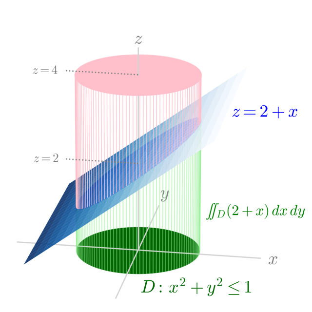
ax.text(1.1, 0, 1,
"$\iint_D (2+x)\,dx\,dy$", c='green',
fontsize="large", ha="left",va="center")
# 切り口
Ndiv = 60
rho = np.linspace(0, 1, Ndiv)
phi = np.linspace(0, 2*np.pi, Ndiv)
x = np.outer(rho, np.cos(phi))
y = np.outer(rho, np.sin(phi))
ax.plot_surface(x, y, f(x, y), fc="blue", ec="blue",
lw = 1, zorder=30)
# ふた
Ndiv = 60
rho = np.linspace(0, 1, Ndiv)
phi = np.linspace(0, 2*np.pi, Ndiv)
x = np.outer(rho, np.cos(phi))
y = np.outer(rho, np.sin(phi))
ax.plot_surface(x, y, zconst(4), fc="pink", ec="pink",
lw = 1, zorder=50)
# 横線
plt.plot([0, -1.2], [0, 0], [2, 2],
c = 'gray', ls='dotted', lw = 1, zorder=50)
ax.text(-1.3, 0, 2, '$z=2$',
c = 'gray', ha='right', va='center')
plt.plot([0, -1.2], [0, 0], [4, 4],
c = 'gray', ls='dotted',lw = 1, zorder=50)
ax.text(-1.3, 0, 4, '$z=4$',
c = 'gray', ha='right', va='center')
ax.set_xlim(-2.5, 2.5)
ax.set_ylim(-2.5, 2.5)
ax.set_zlim(0, 5)
ax.view_init(elev = 20, azim = -80, roll = 0)
ax.axis(False);
plt.savefig("Enchu03.png", dpi=360);
In [8]:
fig = plt.figure(figsize=[6.4, 6.4])
ax = fig.add_subplot(projection='3d')
fig.subplots_adjust(bottom=-0.1,left=0)

# 領域 D
Ndiv = 60
rho = np.linspace(0, 1, Ndiv)
phi = np.linspace(0, 2*np.pi, Ndiv)
x = np.outer(rho, np.cos(phi))
y = np.outer(rho, np.sin(phi))
ax.plot_surface(x, y, zconst(0), fc="darkgreen", ec="darkgreen",
                lw = 0.2, zorder=0)
ax.text(0.3, -1.5, 0,
        "$S = \pi\,r^2 = \pi$", c='darkgreen',
        fontsize="x-large", va="center")

# x 軸
plt.plot([-2,2], [0,0],  [0,0],
         lw = 1, c = "lightgray", zorder=3)
ax.text(2.2, 0, 0, "$x$",
        fontsize="x-large", ha="center", va="center", c='gray')
# y 軸
plt.plot([0,0], [-2,2], [0,0],
         lw = 1, c = "lightgray", zorder=3)
ax.text(0, 2.6, 0, "$y$",
        fontsize="x-large", ha="center", va="center", c='gray')
# z 軸
plt.plot([0,0], [0,0], [0,2], lw = 1, c = "lightgray", zorder=3)
plt.plot([0,0], [0,0], [2,4], lw = 1, c = "lightgray", zorder=4)
plt.plot([0,0], [0,0], [4,4.6], lw = 1, c = "lightgray", zorder=10)
ax.text(0, 0, 4.8, "$z$",
        fontsize="x-large", ha="center", va="center", c='gray')

# 側面を縦線で表してみる
irange = np.linspace(10, -170, 60)
for i in irange:
    phi=np.radians(i)
    xi = np.cos(phi)
    yi = np.sin(phi)
    plt.plot([xi, xi],
             [yi, yi],
             [0, f(xi,yi)],
             c='lightgreen', lw = 0.7, alpha=0.8, zorder=3)
    plt.plot([xi, xi],
             [yi, yi],
             [4, f(xi,yi)],
             c='lightgreen', lw = 0.7, alpha=0.3, zorder=20)

# 切り口
Ndiv = 60
rho = np.linspace(0, 1, Ndiv)
phi = np.linspace(0, 2*np.pi, Ndiv)
x = np.outer(rho, np.cos(phi))
y = np.outer(rho, np.sin(phi))
ax.plot_surface(x, y, f(x, y), color="lightblue",  alpha=0.1,
                lw = 1, zorder=30)

# ふた
Ndiv = 60
rho = np.linspace(0, 1, Ndiv)
phi = np.linspace(0, 2*np.pi, Ndiv)
x = np.outer(rho, np.cos(phi))
y = np.outer(rho, np.sin(phi))
ax.plot_surface(x, y, zconst(4), fc="lightgreen", ec="lightgreen",
                lw = 1, zorder=50)

# 横線
#plt.plot([0, -1.2], [0, 0], [2, 2],
#         c = 'gray', ls='dotted', lw = 1, zorder=50)
#ax.text(-1.3, 0, 2, '$z=2$',
#        c = 'gray', ha='right', va='center')
plt.plot([0, -1.2], [0, 0], [4, 4],
         c = 'gray', ls='dotted',lw = 1, zorder=50)
ax.text(-1.3, 0, 4, '$h=4$', fontsize="x-large",
        c = 'darkgreen', ha='right', va='center')

ax.text(0.3, 1.5, 4.2,
        r"$V=\pi \,r^2 \times h = 4 \pi$", c='darkgreen',
        fontsize="x-large", va="center")
ax.set_xlim(-2.5, 2.5)
ax.set_ylim(-2.5, 2.5)
ax.set_zlim(0, 5)
ax.view_init(elev = 20, azim = -80, roll = 0)
ax.axis(False);
plt.savefig("Enchu04.png", dpi=360);