SymPy による数式処理とグラフ作成
葛西 真寿 弘前大学大学院理工学研究科
この Notebook では,「wxMaxima による数式処理とグラフ作成」のテキストの内容を,Jupyter Notebook 上で Python の SymPy ライブラリを使って説明しています。
セクションの構成は,wxMaxima 版のテキストに準じています。
ですからこの Notebook は,一から SymPy を始めようとしている人だけでなく,Maxima は知っているが同じことを SymPy ではどのように計算するかということに興味を持っている人にも参考になるのではないかと思います。
SymPy による数式処理
基本操作
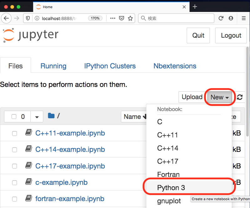
Jupyter Notebook の起動
ターミナル(コマンド プロンプト,Windows PowerShell 等)で
jupyter notebook (または jupyter-notebook)
右上の「New」から 「Python 3」を選ぶ。
計算の実行と改行
計算の実行は,数値や式などを入力して 最後に Shift キーを押しならが Enter キーを押します。
まずは簡単なかけ算 $123 \times 456$ を計算してみます。
123 * 456
2 の 100 乗 ($2^{100}$) のような大きい数でも,厳密な結果を出力します。(** は累乗を表します。^ ではありません。)
2**100
float 関数を使って不動小数点表示で近似値を出力させることもできます。
float(2**100)
ここまでは Python の標準の機能だけで計算できました。
sympy の import
これからは,微分・積分などの記号計算(いわゆる数式処理)を行うためのライブラリ SymPy が必要です。以下のようにします。
from sympy.abc import *
from sympy import *
init_printing()
積分 $\displaystyle \int 3 x^2\, dx$ の計算をしてみます。
integrate(3*x**2, x)
計算結果の保存と読み込み
Jupyter Notebook (の SymPy)で計算した結果を保存するには,「File」メニューから「Save as ... 」でファイル名をつけて保存します。
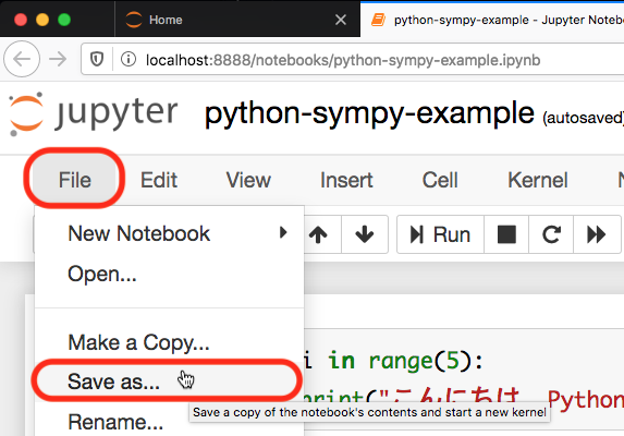
「File」メニューの真下に,なにやら四角で右上隅がかけている形のアイコンがありますが(これが「フロッピーディスク」というものであることは,20世紀の昔を知る人にしかわからないと思います),このアイコンをクリックしても保存されます。
![]()
また,「File」メニューから「Open... 」を選び,計算結果が保存された Notebook をまた利用することもできます。
表記などの約束事
コメント(実行に影響しない注釈)を入れたいときは,コメントにしたい部分を # ではじめます。
1 + 2 + 3
1 + 2 # + 3
足し算 +,引き算 -,かけ算 *,割り算 / における優先順位は数学と同じです。優先して計算したい箇所は ( ) で囲みます。
1 + 2 * 3
(1 + 2) * 3
代入
変数に式や値を代入するときは,等号 = を使います。
変数 a に $100 + 3/21$ を代入し,a の値を表示させる例です。
a = 100 + 3/21
a
上記の計算では,割り算 / は実数になります。有理数として分数をあつかう際は,Rational を使います。
a = 100 + Rational(3,21)
a
この a を使って計算を続けます。
(a - 100) * 7
変数 eq に式 $x^2 + 3 x + 2$ を代入します。
eq = x**2 + 3*x + 2
eq
eq を factor 関数で因数分解します。
factor(eq)
関数の定義
Python の記法で関数を定義します。$f(x) = x^2$
def f(x):
    return x**2
f(x)
$f(4) = 4^2 = 16$
f(4)
$f(3\sqrt{A}) = (3\sqrt{A})^2 = 9 A$
f(sqrt(A)*3)
$\frac{d}{dx}(x \cos x)$ を計算します。
diff(x*cos(x), x)
微分した結果を関数 g(x) として定義する例。
def g(x):
    return diff(x*cos(x), x)
g(x)
でも,上記のような導関数の定義だと,ちょっと困る。それは...
g(x) が関数として定義されていれば,たとえば
$$ g(1) = -1 \times \sin (1) + \cos(1) $$となるはずですが...
# g(1)
上記の # を取って実行するとエラーになります。そこで...
def f(x):
    return x*cos(x)
def df(x1):
    return diff(f(x), x).subs(x,x1)
df(1)
integrate(df(x), x) == f(x)
上の例では,以下の計算をしています。
$$f(x) \equiv x \cos x, \quad df(x) \equiv \frac{d}{dx} f(x), \quad \int df(x) \ dx = f(x) $$実行結果の表示・非表示
x**2 + 3*x + 2
代入や定義のときは,式や変数の値が表示されません。
eq = x**2 + 3*x + 2
明示的に変数を Shift + Enter すれば表示されますが,文末に ; をつけると結果が出力されません。
eq
eq;
前の出力結果の参照
直前の出力結果は _ で参照できます。
expand((x - 2)**4)
factor(_)
expand(_)
一時的代入
c = 2*x
c
subs 関数を使うことで,一時的に変数に値を代入することができます。
c.subs(x,3)
c の定義そのものは変わりません。
c
リスト成分の取り出し
$f(x) = x^2 + 3 x + 2$ を定義します。
def f(x):
    return x**2 + 3*x + 2
solve で方程式 $f(x) = 0$ を解きます。2次方程式ですから,解は2個,リストとして出力されます。
sol=solve(f(x), x)
sol
Python では,ゼロはじまりですから,最初のリスト成分は sol[0],次が sol[1] です。
sol[0], sol[1]
解を代入して,確かに $f(x_0) =0, f(x_1) = 0$ となっていることを確認します。
f(sol[0]), f(sol[1])
数の計算・基本的な関数
基本的な演算
1 から 10 までの和を求めてみます。
1 + 2 + 3 + 4 + 5 + 6 + 7 + 8 + 9 + 10
同様の計算は,公式 $\displaystyle \frac{n(n+1)}{2}$ で $ n=10 $ として求めることもできます。
(n*(n + 1)/2)
(n*(n + 1)/2).subs(n,10)
(n*(n + 1)/2)
$2^4$ の計算。累乗は ** で表します。
2**4
$4$ の階乗の計算をします。$4! = 4\times 3\times 2\times 1 = 24$ です。SymPy では,階乗は factorial 関数を使います。
factorial(4)
factorial2 関数は,一つおきの会場の計算をします。$5!! = 5\times 3\times 1 = 15$ です。
factorial2(5)
練習
(練習) $3, 2, 1$ でつくる最大の数
数字の 3 と 2 と 1 を1個ずつ使った演算でつくることができる最大の整数は?
(ヒント)
$(1+2)\times 3 = 9$ では全然ダメ。そのまま並べると,$321$ ですが,累乗を使うともっと大きい数をつくることができるでしょう。
$21^3$ とか,$31^{2}$ とか,$2^{31}$ とか,$3^{21}$ とか...
基本的な定数
I, pi, E の import
SymPy の基本的定数は,以下のようにして import して使います。
from sympy import I, pi, E
| 円周率 $\pi$ | 無限大 $\infty$ | 自然対数の底 $e$ | 虚数単位 $i$ |
|---|---|---|---|
pi |
oo |
E |
I |
人類の至宝,オイラーの等式 $e^{i \pi} = -1$
E**(I * pi)
pi
近似値を表示するには,float 関数や Float 関数を使います。
float(pi)
Float 関数で 32桁まで円周率 $\pi$ を表示する例です。
Float(pi,32)
基本的な関数
| 平方根 | 指数関数 | 自然対数 | 絶対値 | 三角関数 | 逆三角関数 | 双曲線関数 |
|---|---|---|---|---|---|---|
sqrt |
exp |
ln (=log) |
abs |
sincostan |
asinacosatan |
sinhcoshtanh |
うっかり $\sqrt{x^2} = x$ としないように。$x$ が実数なら $\sqrt{x^2} = |x|$ です。が...
sqrt(x**2)
$x$ を実数と assume してやることで,
x=Symbol('x', real=True)
sqrt(x**2)
ピタゴラスの定理をみたす3つの整数の例。$\sqrt{3^2 + 4^2} = 5$ ですね。
sqrt(3**2 + 4**2)
$\exp(1) = e^1 = e$ のこと。
exp(1) - E
以前,変数 a に値を入れたりしていると困るので,念のために a=Symbol("a") として変数の初期化を行います。
a=Symbol("a")
exp(log(a))
$\log e^2 = 2 \log e = 2$
log(E**2)
練習
(練習) ピタゴラス数
$a^2 + b^2 = c^2$ をみたす正の整数の組をピタゴラス数といいます。
ピタゴラス数は2つの任意の正の整数 $m, n$ から以下のようにして何組でもつくることができます。
$$ a = |m^2 - n^2|, \quad b=2mn, \quad c = \sqrt{a^2 + b^2} $$このとき,$c$ は(平方根をとるのにもかかわらず)必ず整数になることを示しなさい。
試しに少し数値実験してみます。
念のため,m と n の変数を初期化して,a, b, c を m と n を使って表します。
m = Symbol("m")
n = Symbol("n")
a = abs(m**2 - n**2)
b = 2*m*n
c = sqrt(a**2 + b**2)
c
m と n に 1 から 100 までのランダムな整数をふって,c の値がいくらになるか計算してみます。
import random
c.subs([(m,random.randint(1,100)), (n,random.randint(1,100))])
c.subs([(m,random.randint(1,100)), (n,random.randint(1,100))])
c.subs([(m,random.randint(1,100)), (n,random.randint(1,100))])
$c = \sqrt{a^2 + b^2}$ は確かに整数になっています。証明も簡単ですね。
参考
random.randint(1,100) は 1 から 100 までのランダムな整数を与えます。random.random() ならどうなるか,試してみましょう。
練習
(練習) 星の明るさと等級
夜空に見える星の見かけの明るさ $L$ は等級 $m$ で表わされ,以下のような関係があります。
$$ m = -2.5\log_{10} L + \mbox{定数} $$1等星と6等星では,どちらのほうが何倍明るいですか。
(ヒント)
1等星と6等星の見かけの明るさをそれぞれ,$L_1,\ L_6$ とすると,
$$1 = -2.5\log_{10} L_1 + \mbox{定数}, \quad 6 = -2.5\log_{10} L_6 + \mbox{定数} $$両辺を引くと,
$$ 1 - 6 = -2.5 (\log_{10} L_1 - \log_{10} L_6) $$つまり,
$$ \log_{10} \frac{L_1}{L_6} = \frac{-5}{-2.5} = 2 $$常用対数 $\log_{10}$ は以下のようにして使います。
log10 の import
from sympy.codegen.cfunctions import log10
log10(100)
三角関数の値・引数の単位
三角関数の値を数値で求めたいときには,以下のようにします。
$$\sin \frac{\pi}{3} = \frac{\sqrt{3}}{2}$$sin(pi/3)
float 関数を使って,直前の結果を浮動小数点表示します。
float(_)
あるいは,変数 Pi に浮動小数点数の $\pi$ の値を代入します。
Pi=float(pi)
sin(Pi/3)
上の例では,浮動小数点数を入れると,sin も浮動小数点表示で答えを返します。
三角関数の引数の単位はラジアンです。度を使って求めたいときは以下のようにします。
$60^{\circ}$ をラジアンに直した値 $\displaystyle 60 \times \frac{\pi}{180}$ を使って計算します。
sin(Rational(60, 180)*pi)
度をラジアンに変数関数 degrad を定義します。
def degrad(x):
    return Rational(x, 180)*pi
degrad(60) を引数にして sin の値を求めます。
sin(degrad(60))
練習
(練習) 屋根勾配
日本の大工さんは,家の屋根の勾配は角度ではなく,伝統的に3寸勾配,4寸勾配のように水平方向に1尺(10寸)に対して垂直方向に何寸立ち上がるかで示します。
(本当です。実際に家を建てた本人が言っているのだから間違いないです。)
下図のログハウスの屋根は8寸勾配です。傾斜角度にすると何度ですか?
(大工さんは8寸勾配と言いますが,照明器具を設置する電気屋さんは8寸勾配ではなく,傾斜角は何度だ?と聞きますので,この変換が必要でした。)

ラジアンを度に変換する関数を作っておきます。
def raddeg(x):
    return float(x * 180/pi)
x = Symbol('x')
# 一寸勾配
x = 0.1
Float(atan(x), 3), Float(raddeg(atan(x)), 5)
# 二寸勾配
x = 0.2
Float(atan(x), 3), Float(raddeg(atan(x)), 5)
以下に各寸勾配を角度で表した表があります。10寸勾配(矩勾配 かねこうばい)まで表を完成させましょう。
| 勾配 | 1寸勾配 | 2寸勾配 | ... |
|---|---|---|---|
atan(0.1) |
atan(0.2) |
... | |
| ラジアン | 0.0997 | 0.197 | ... |
| 度 | 5.7106° | 11.310° | ... |
数列の和
数列の和の計算する関数 summation の書式は,
summation(一般項 a_i, (i, 初めの i, 最後の i)) です。
summation(i**2, (i, 1, 10))
一般の $N$ までの数列の和
$$\sum_{i=1}^{N} i^2 = \frac{N (N+1)(2 N + 1)}{6}$$summation(i**2, (i, 1, N))
factor(_)
練習
(練習) 数列の和
- 初項 $a_1$,公差 $d$ の等差数列の第1項から第$n$項までの和を求めよ。
- 初項が 3,公比が 2 の等比数列について,第10項までの和を求めよ。
- $\sum_{i=1}^{n} b_1 r^{i-1}$ を求めよ。また無限等比数列の和 $n \rightarrow \infty$ を求めよ。ただし,$0 < r < 1$。
(ヒント)
1.は,以下のような計算。文末に ; をつけると,結果が表示されません。
a1 = Symbol('a1')
summation(a1 + ( i- 1)*d, (i, 1, n));
b1 = Symbol('b1')
sum2 = summation(b1*r**(i - 1), (i, 1, n))
sum2
関数のテイラー展開
$\sin x$ を $x=0$ のまわりで $x^5$ の項までテイラー展開する例。
(Python はゼロからはじまるから,$x^5$ は$x^0$ から数えて6番目,と覚えておけばいいのかなぁ... )
x = Symbol('x', real=True)
series(sin(x), x, 0, 6)
$e^{i x}$ ($i$ は虚数単位)のテイラー展開
series(exp(I*x), x, 0, 6)
その虚部を im 関数でとると...
(ちなみに,実部は re です。)
im(_)
$\cos x, \tan x$ 等のテイラー展開もやってみましょう。
式の整理・簡単化
SymPy では,多項式やいろいろな関数を含んだ式の変形や整理・簡単化が可能です。
展開・因数分解・簡単化
$(x+1)^2$ を展開します。
expand((x + 1)**2)
$x^3-1$ を因数分解します。
factor(x**3 - 1)
$\frac{3}{x^3-1}$ を部分分数に展開する例。
apart(3/(x**3 - 1))
simplify (この場合は ratsimp でも可)を使って,上式を「簡単化」します。
simplify(_)
三角関数を含む式の簡単化
三角関数や双曲線関数を含む式の簡単化には trigsimp を使います。
$\cos^2 x - \sin^2 x$ を「簡単化」します。
trigsimp(cos(x)**2 - sin(x)**2)
$\cosh^2 x - \sinh^2 x$ を「簡単化」します。
trigsimp(cosh(x)**2 - sinh(x)**2)
$\cos 3 x$ を展開してみます。
expand(cos(3*x), trig=True)
simplify(_)
練習
(練習) 加法定理・三倍角の公式
- 三角関数および双曲線関数の加法定理を確認しなさい。
- $\sin 3 x$ を $\sin x$ だけを使って表しなさい。また,$\tan 3x$ を$\tan x$ だけを使って表しなさい。
(ヒント)
$\sin (x + y)$ を以下のように展開 (expand) して加法定理を確認することができます。
双曲線関数についても、trig = True をつけて展開してみてください。
expand(sin(x + y), trig=True)
expand(sinh(x + y), trig=True);
微分・積分・数値積分
微分・積分を行う関数の表記を以下に示します。
| 操作 | 表記例 |
|---|---|
| 微分 | diff(f, x) |
| n 階微分 | diff(f, x, n) |
| 不定積分 | integrate(f, x) |
| 定積分 | integrate(f, (x, a, b)) |
微分・積分
$x^3 + 5 x + 2$ を $x$ で微分します。
$$\frac{d}{dx} \left(x^3 + 5 x + 2\right)$$diff(x**3 + 5*x + 2, x)
$x^3 + 5 x + 2$ を $x$ で2階微分します。
$$\frac{d^2}{dx^2} \left(x^3 + 5 x + 2\right)$$diff(x**3 + 5*x + 2, x, 2)
$x^2 \cos x + 2 x \sin x$ を $x$ で積分します。
$$\int \left(x^2 \cos x + 2 x \sin x \right)\, dx$$integrate(x**2 * cos(x) + 2*x*sin(x), x)
定積分の例です。
$$\int_0^{\pi/2} \sin x \,dx = 1$$integrate(sin(x), (x, 0, pi/2))
練習
(練習) 関数の傾き
$\displaystyle y = \frac{2x-1}{x+1}$ が $x \neq -1$ で増加関数であることを示しなさい。
(練習) 積分
次の積分を計算しなさい。
$$\mbox{1.}\ \int e^x \sin x\ dx, \qquad\mbox{2.}\ \int \frac{x^2-2x-2}{x^3-1}\, dx $$integrate((x**2-2*x-2)/(x**3-1),x)
数値積分
解析的に積分できない場合は,数値積分によって近似値を求めることができます。
$\displaystyle \int_0^{\pi} \sin(\sin x) \,dx$ の計算をします。解析的に解けないとそのままで返します。
integrate(sin(sin(x)), (x, 0, pi))
_.evalf()
$\displaystyle \int_0^1 e^{-x^2}\,dx$ の数値積分
integrate(exp(-x**2), (x, 0, 1)).evalf()
ちなみに,ガウス積分は...
integrate(exp(-x**2), (x, 0, oo))
Eq(Integral(exp(-x**2), (x, 0, oo)),
   Integral(exp(-x**2), (x, 0, oo)).doit())
方程式
多項式方程式・連立方程式
Sympy では、式の計算だけでなく、代数方程式を解くことができます。例を以下に示します。
$x^2 + 2 x - 2 = 0$ を $x$ について説きます。
solve(x**2 + 2*x -2, x)
連立方程式
$$x^2 + y^2 = 5, \quad x + y =1$$を $x, y$ について解きます。
solve([x**2 + y**2 - 5, x + y -1], [x, y])
3次方程式 $x^3 = 8$ を解きます。
x = Symbol('x')
sols = solve(x**3-8)
sols
念のため,3番目の答えを3乗して簡単にすると...
sols[2]**3
simplify(_)
実数解のみを求める場合は,real_roots を使います。
また,変数 x を実数として solve を使うという手もあります。
real_roots(x**3 - 8)
x = Symbol('x', real=True)
solve(x**3-8)
練習
(練習) 鶴と亀と蟻
鶴と亀と蟻,個体数の合計は10。足の数は全部で34本。蟻は亀より1匹少ない。鶴,亀,蟻はそれぞれ何羽・何匹?
鶴・亀・蟻の個体数をそれぞれ $x, y, z$ として連立方程式を立てて solve します。蟻の足は何本かわかりますよね?
かつて線形代数の授業でこの問題を出したとき,真っ先に出た質問が「先生,蟻の足は何本ですか?」でした... orz
方程式の数値解
1変数多項式方程式の数値解を求めてみます。
関数 $f(x) = x^3 + 8 x -3$ を定義します。
def f(x):
    return x**3 + 8*x -3
$f(x) = 0$ の全数値解を求めます。
sols = solve(f(x))
for sol in sols:
    print(sol.evalf())
念のために,3つ目の数値解 $x_3$ を使って $f(x_3)$ が $0$ になるのかを確かめてみます。
x3 = float(sols[2])
x3
f(x3)
浮動小数点にしないでも,$f(x_3)$ が $0$ になることは以下のようにしても確かめることができます。
f(sols[2]);
simplify(_)
多項式方程式でない場合は,nsolve 関数を使って数値解を探します。
関数 $g(x) = (x-1) e^x$ の定義。
def g(x):
    return (x - 1)*exp(x)
$g(x) - 1 = 0$ の解は solve では明示されません。
solve(g(x) - 1)
nsolve 関数を使って,$x = 1$ のあたりからはじめて20桁の精度で数値解を求める例。
nsolve(g(x) - 1, x, 1, prec=20)
出た数値解を代入して確かめると...
g(_)
練習
(練習) 関数の極大値
次の関数が極大値をとる 𝑥 の値およびその極大値を求めよ。
$$ 1. \ \ \frac{x^3}{e^x -1} \qquad 2. \ \ \frac{x^5}{e^x -1}$$1階常微分方程式の例
SymPy では dsolve を使って常微分方程式解きます。
1階常微分方程式 $\displaystyle \frac{dy}{dx} = a y$ を解きます。
y = Function('y')(x)
a = Symbol('a')
eq = Eq(Derivative(y, x), a*y)
eq
dsolve(eq, y)
上の例では,$C_1$ は(任意の)積分定数です。
初期条件を与えると,積分定数の値は決まります。以下は,$x = 0$ で $y(0) = 1$ という初期条件を ics={...:...} の形に与えて dsolve します。この初期条件によって $C_1 = 1$ と決まった解が表示されます。
dsolve(eq, y, ics={y.subs(x,0):1})
2階常微分方程式の例
2階常微分方程式 $\displaystyle \frac{d^2 x}{dt^2} = -K x$ (ただし $K > 0$)を解く例を示します。
これは単振動の運動方程式で,おそらく大学生になったら最初に出会う微分方程式です。
x = Function('x')(t)
K = Symbol('K', positive = True)
eq = Eq(Derivative(x, t, 2), -K*x)
eq
dsolve(eq, x)
上のように,2つの積分定数 $C_1, C_2$ を含む一般解が表示されました。
初期条件として,初期時刻 $t = 0$ における初期位置を $x(0) = x_0$,初速度を $\dot{x}(0) = v(0) = v_0$ として,この運動方程式を解くと...
x0 = Symbol('x0')
v0 = Symbol('v0')

ans = dsolve(eq, x,
      ics = {x.subs(t, 0):x0,
             diff(x, t).subs(t, 0):v0}
      )
ans
ちなみに,$K \rightarrow 0$ の極限で,この解はばねの復元力を受けない等速直線運動になるはずです。
分母に $\sqrt{K}$ があるので,$K = 0$ にしたら大変なことになるのでは?と一瞬思いますが,極限をとって確認してみると...
def x(t):
    return ans.rhs
x(t)
$\displaystyle \lim_{K \rightarrow 0} x(t) = ...$
limit(x(t), K, 0)
$\displaystyle \lim_{K \rightarrow 0} \frac{dx}{dt} = ...$
limit(diff(x(t), t), K, 0)
最初から $K=0$ とした微分方程式 $\displaystyle \frac{d^2x}{dt^2}=0$ を解いても同じ答えが(当然)出てきます。
x = Function('x')(t)
dsolve(Derivative(x, t, 2), x,
       ics = {x.subs(t, 0):x0,
              diff(x, t).subs(t, 0):v0}
      )
練習
(練習) 一様重力場中の投げ上げ運動
- 時刻 $t=0$ に高さ $0$ から初速度 $v_0$ で鉛直上方に投げ上げた物体の時刻 $t$ における高さ $y(t)$ を求めなさい。運動方程式は以下の通り。 $$\frac{d^2 y}{dt^2} = - g$$ ただし,$g$ は重力加速度の大きさで,定数である。
- 速度に比例する空気抵抗がある場合,運動方程式は以下のようになる。 $$\frac{d^2 y}{dt^2} = - g - \beta\frac{dt}{dt}$$ ここで,$\beta$ は定数。前問と同じ初期条件のときに $y(t)$ を求めなさい。
- 前問2.で求めた解について, $\beta \rightarrow 0$ のときに前問1. の答えに一致するかどうか,確かめなさい。
ベクトルと行列
3次元ベクトルの表記
3次元ベクトル $\boldsymbol{a} = (a_1, a_2, a_3)$ の表記例(成分は実数とします)。
a1, a2, a3 = symbols('a1 a2 a3', real=True)
a = Matrix([a1, a2, a3])
a
$\boldsymbol{b}$ も同様ですが,以下のように少し簡単化した表記もできます。
b = Matrix(symbols('b1:4', real=True))
b
ベクトルの内積
ベクトルの内積 $\boldsymbol{a}\cdot\boldsymbol{b}$ には .dot() を使います。
a.dot(b)
ベクトル $\boldsymbol{a}$ の大きさ $|\boldsymbol{a}|$ は以下のように .norm() を使います。
a.norm()
$|\boldsymbol{a}| = \sqrt{\boldsymbol{a}\cdot \boldsymbol{a}}$ です。
a.norm() == sqrt(a.dot(a))
ベクトルの外積
3次元ベクトル同士の外積 $\boldsymbol{a}\times \boldsymbol{b}$ は .cross() を使います。
a.cross(b)
練習
(練習) ベクトルの内積,外積
$\displaystyle \boldsymbol{a} = \left(-\frac{1}{\sqrt{2}}, \frac{1}{\sqrt{2}}, \sqrt{3}\right), \quad \boldsymbol{b} = \left(-1, 1, -\sqrt{2}\right)$ について以下の量を計算しなさい。
$$1.\ |\boldsymbol{a}|, \quad 2.\ |\boldsymbol{b}|, \quad 3.\ \boldsymbol{a}\cdot \boldsymbol{b}, \quad 4.\ \boldsymbol{a}\times \boldsymbol{b} $$また,2つのベクトル $\boldsymbol{a}, \boldsymbol{b}$ のなす角を $\theta$ としたときの $\cos\theta$ および $\sin\theta$ を求めなさい。
(練習) ベクトルの3重積
- スカラー3重積の以下の性質を確かめなさい。 $$\boldsymbol{a}\cdot (\boldsymbol{b}\times\boldsymbol{c}) = \boldsymbol{b}\cdot (\boldsymbol{c}\times\boldsymbol{a}) = \boldsymbol{c}\cdot (\boldsymbol{a}\times\boldsymbol{b}) $$
- ベクトル3重積の以下の性質を確かめなさい。 $$\boldsymbol{a}\times (\boldsymbol{b}\times \boldsymbol{c}) = (\boldsymbol{a}\cdot \boldsymbol{c})\boldsymbol{b} - (\boldsymbol{a}\cdot \boldsymbol{b}) \boldsymbol{c} $$
行列の簡単な計算
2行2列の行列 $A$ の定義。(念のため,行列の成分に使う変数は初期化しておきます。)
a, b, c, d = symbols('a b c d')

A = Matrix([[a, b],
            [c, d]])
A
transpose(A) は転置行列 $A^T$。
transpose(A)
det は行列式。
det(A)
$A$ の逆行列$ A^{-1}$ は A**(-1) のように書きます。
A**(-1)
$A^{-1} A$ が単位行列になることを確かめます。行列の積は * で表します。
A**(-1)*A
simplify(_)
3次元の回転行列 $O$ の定義。
O = Matrix([[cos(theta), -sin(theta), 0],
            [sin(theta),  cos(theta), 0],
            [0,           0,          1]])
O
この行列 $O$ が直交行列(転置行列が逆行列)であることを示します。 そのためには,$O O^T$ が単位行列であることを示せばよいです。
O*transpose(O)
simplify(_)
3次元ベクトル $\boldsymbol{r} = (x_1, x_2, x_3)$ をこの回転行列で直交変換します。
r = Matrix(symbols('x1:4'))
r
O*r
練習
(練習) 直交変換されたベクトルの大きさ
直交変換されたベクトル $\boldsymbol{r}^{\prime} = O \boldsymbol{r}$ の大きさは,もとのベクトル $\boldsymbol{r}$ の大きさと同じであることを示しなさい。
ヒント:例えば以下のように...
(O*r).dot(O*r);
simplify(_);
(練習) 逆行列の転置行列と転置行列の逆行列
$\displaystyle \left(A^{-1}\right)^T = \left( A^T \right)^{-1}$ を示しなさい。
ヒント:例えば,3次正方行列 $A$ を以下のように定義して...
A = Matrix([symbols('a11:14'),
            symbols('a21:24'),
            symbols('a31:34')])
A
直接 $\displaystyle \left(A^{-1}\right)^T - \left( A^T \right)^{-1}$ を計算して $0$ になるか調べてみましょう。
transpose(A**(-1)) - transpose(A).inv();
simplify(_);
Sympy や Matplotlib によるグラフ作成
2次元グラフ plot の例
2次元グラフ $y = f(x)$ を $a \le x \le b$ 範囲で描く一般的な表記は
plot(f(x), (x, a, b)) です。
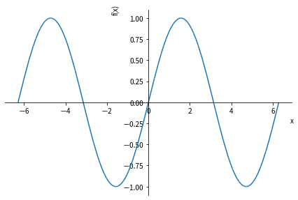
例として,$y = \sin x$ のグラフを $-2\pi \le x \le 2 \pi$ の範囲で描きます。基本的な定数の一つである円周率 $\pi$ は SymPy では pi と書くのでしたね。
from sympy import *
from sympy.abc import *
from sympy import I, pi, E
plot(sin(x), (x, -2*pi, 2*pi));
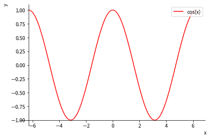
いくつかオプションを指定して描く例です。
以下では,座表軸の交点の位置を $(-2\pi, -1)$ に設定し,線の色(line_color)を赤にし,凡例(legend)を表示させ,x軸とy軸にラベルを表示させて $y=\cos x$ を描いています。
plot(cos(x), (x, -2*pi, 2*pi),
     axis_center=(-2*pi, -1),
     line_color='red',
     legend=True,
     xlabel='x',
     ylabel='y');
figsize, font.size の変更と SVG 表示
以下のように plot すると,グラフのサイズが小さめで,なんか滲んで見えます。
plot(sin(x), title='タイトル', xlabel='横軸', ylabel='縦軸');
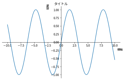
Full HD くらいでは違いがわからないかもしれませんが,高解像度(いわゆる Retina)ディスプレイだとショボく見えるので svg 表示にし,グラフの大きさも少し大きめにしてみます。
import matplotlib.pyplot as plt
plt.rcParams['figure.figsize'] =8,6
plt.rcParams['font.size'] = 12
from IPython.display import set_matplotlib_formats
%matplotlib inline
set_matplotlib_formats('svg')
plot(sin(x), title='タイトル', xlabel='横軸', ylabel='縦軸');
3次元グラフ plot3d の例
3次元グラフ $z = g(x, y)$ を描く一般的な表記例は plot3d(g(x,y), (x, a, b), (y, c, d)) です。plot3d を使うためには,以下のように最初に import する必要があります。
plot3d の import
from sympy.plotting import plot3d
x, y = symbols('x y') # 念のため,以下で使う変数 x, y を初期化
例として,$z = x \sin y$ のグラフを $-3 \le x \le 3$,$-4 \le y 4$ の範囲で描きます。
plot3d(x*sin(y), (x, -3, 3), (y, -4, 4), xlabel='x', ylabel='y');
数値データのグラフ作成例
Python でリスト形式の離散的な数値データをグラフに描く際,SymPy に適当な関数がないようなので,matplotlib.pyplot を import して使ってみます。
matplotlib.pyplot の import
import matplotlib.pyplot as plt
以下の例では,リスト x の値をx座標の値,対応するリスト y の値をy座標の値として6個の点をつないだ折れ線グラフを描きます。
x = [i for i in range(6)]
y = [i**2 for i in x]
print(x)
print(y)
plt.plot(x, y);
オプションを設定してプロットする例。ここでは,フォーマットを + にして線でつながずに描きます。オプションのマーカーフォーマットには '+'(プラスマーカー)の他にも,'.'(点),'ro'(赤丸)など,線種には,'-'(実線),'--'(ダッシュ),':'(ドット)などがあります。
plt.plot(x, y, '+');
複数のグラフを重ねて表示
SymPy で複数のグラフを重ねて表示する例を示します。
$y = x^2 - 1$ と $y = 4 x - 5$ の2つのグラフを重ねて描きます。$x$ の範囲は $-5 \le x \le 5$ です。
x = Symbol('x')  # 念のため,変数 x を初期化
plot(x**2 - 1, 4*x - 5, (x, -5, 5));
いくつかオプションを設定して描く例です。以下の例では,縦軸(y軸)の表示範囲を ylim で制限して表示します。
p= plot(x**2 - 1, 4*x - 5, (x, -5, 5),
        ylim=(-5, 10), legend=True, show=False);
p[0].line_color='b'
p[1].line_color='r'
p.show()
上のグラフをみると,2つのグラフは1点で接しているように見えます。実際に確かめてみます。
# y = x**2 -1 と y = 4*x - 5 が交差または接している点の x 座標
def f(x):
    return x**2 - 1
def g(x):
    return 4*x - 5
# f(x) = g(x) をみたす x を求める。
sol = solve(Eq(f(x), g(x)), x)
sol
# 解が1個なので接していることがわかった。その接点の座標は...
x0 = sol[0]
y0 = f(x0)
x0, y0
# 接線の傾き
def df(x1):
    return diff(f(x), x).subs(x, x1)
df(x0)
# 接線の方程式は
x, y = symbols('x y')
Eq(y, df(x0)*(x - x0) + y0)
練習
(練習)
以上のことができたら,$y = x^2 -1$ の $x = 1$ や $x = 1/2$ 等の点における接戦のグラフも描いでみましょう。
数値データを読み込む
Python では,あらかじめ作成された数値データファイルを読み込んでグラフを描くこともできます。
以下のような内容のファイル test.dat がカレント・ディレクトリ ./ にあるとします。
# x   y
  0   0
  1   1
  2   4
  3   9
  4   16
  5   25
numpy の import
データファイルを読み込む関数は,SymPy では見当たらないようなので,numpy を import し,loadtxt を使用します。
import numpy as np
data = np.loadtxt('./test.dat')
print(data)
matplotlib の plot でグラフを描くために,x座標値のリストと,対応するy座標値のリストを(以下の例では x1 および y1 としt)準備します。
x1 = [data[i,0] for i in range(len(data))]
y1 = [data[i,1] for i in range(len(data))]
すでに import matplotlib.pyplot as plt しているかと思いますが,念のためにあらためて import しておきます。SymPy の plot ではなく,matplotlib の plot ですよ。以下の例では 'bo' オプションをつけて青丸で描いています。
import matplotlib.pyplot as plt
plt.plot(x1, y1, 'bo');
数値データと理論曲線を重ねて表示
前節の数値データファイル test.dat と理論曲線 $y = x^2$ の2つのグラフを重ねて表示してみます。
SymPy 単独で描く方法が思い当たらないので,matplotlib と numpy のお世話になります。
import matplotlib.pyplot as plt
import numpy as np

# test.dat の x1, y1 は前節で定義済み。
plt.plot(x1, y1, 'bo', label='data');   # test.dat の x1, y1 を青丸で plot

# y = x**2 のデータをここで作成。
x = np.arange(0, 5.2, 0.2)
y = x**2
plt.plot(x,  y,  '-r', label='$y=x^2$'); # y = x**2 を赤線で plot
plt.legend();                            # label で定義しておいた判例を表示
媒介変数表示の2次元グラフ
半径1の円の方程式は $x^2 + y^2 = 1$ です。
この円を描くには,$y = \pm\sqrt{1-x^2}$ として $y = f(x)$ の形にするよりも,以下のような媒介変数表示にしたほうが簡単でしょう。
$$ x = \cos t, \quad y = \sin t, \quad(0 \le x \le 2\pi)$$このような媒介変数表示の2次元グラフを SymPy で描くには以下のようにします。
plot_parametric(cos(t), sin(t), (t, 0, 2*pi));
これは媒介変数表示の円のグラフですが,横につぶれて楕円のように見えます。せっかくですから,グラフの縦横の比を$1:1$にして円らしく見えるようにします。
aspect_ratio というオプションがありますが,効かないようです。
import matplotlib.pyplot as plt
# デフォルトでは plt.rcParams['figure.figsize'] = (6.0, 4.0) だった
plt.rcParams['figure.figsize'] = (5, 5)
plot_parametric(cos(t), sin(t), (t, 0, 2*pi), xlim=(-1.1, 1.1), ylim=(-1.1, 1.1));
練習
(練習) 楕円のグラフ(楕円中心を原点として)
同様にして,楕円のグラフを描くこともできます。原点を中心とし,長半径 $a$,短半径 $b$ の楕円の式は
$$ \frac{x^2}{a^2} + \frac{y^2}{b^2} = 1 $$です。媒介変数表示では,
$$ x = a \cos t, \quad y = b \sin t \quad (0 \le t \le 2\pi)$$と書けます。$a, b$ に適当な値を入れて楕円のグラフを描きなさい。
参考:陰関数のままグラフ化
SymPy では,$x^2 + y^2 = 1$ を $y$ について解いたり,媒介変数表示したりしなくても,plot_implicit を使えばそのままグラフを描くことができます。
x, y = symbols('x y')
eq = Eq(x**2 + y**2, 1)
eq
x, y = symbols('x y')
plt.rcParams['figure.figsize'] = (5, 5)
plot_implicit(eq, (x, -1, 1), (y, -1, 1));
海王星と冥王星の軌道
焦点を原点とした楕円のグラフ
太陽からの万有引力を受けて運動する惑星(惑星だけでなく,準惑星や小天体も含みます)は,太陽を焦点とした楕円軌道を描きます。焦点を原点とし,長半径 $a$,離心率 $e$ の楕円の方程式は,極座標 $r, \phi$ を使って以下のように表すことができます。
$$ r = \frac{a(1-e^2)}{1 + e\cos \phi}$$さて,かつては第9惑星,現在では準惑星の一つである冥王星も楕円軌道を描きます。冥王星の軌道長半径 $a_P = 39.767 \,\mbox{au}$,離心率 $e_P = 0.254$ を使って冥王星の軌道を描きます。
まず,極座標表示の楕円の式を関数として定義します。
def r(a, e, phi):
    return a*(1-e**2)/(1 + e*cos(phi))
import matplotlib.pyplot as plt
# デフォルトでは plt.rcParams['figure.figsize'] = (6.0, 4.0) だった
plt.rcParams['figure.figsize'] = (6, 6)
aP = 39.767
eP = 0.254
plot_parametric(r(aP,eP,phi)*cos(phi), r(aP,eP,phi)*sin(phi),
                (phi, 0, 2*pi), xlim=(-50,50), ylim=(-50,50));
では,この冥王星の軌道と,その内側をまわる海王星の軌道を重ねて描いてみましょう。
海王星の軌道長半径は $a_N=30.1104\,\mbox{au}$,離心率は $e_N=0.0090$ と小さいので簡単のために $e_N = 0$ として扱います。実際の2つの天体の軌道は同じ平面上にありませんが,太陽からの距離のみをみるために,ここでは同一平面上に描きます。
aN = 30.1104
eN = 0
p = plot_parametric((r(aP,eP,phi)*cos(phi), r(aP,eP,phi)*sin(phi)),
                    (r(aN,eN,phi)*cos(phi), r(aN,eN,phi)*sin(phi)),
                    (phi, 0, 2*pi), xlim=(-50, 50), ylim=(-50, 50), show=False)
p[0].line_color='b'
p[1].line_color='r'
p.show()
さて,この冥王星と海王星の軌道のグラフをみると,軌道が交差しているように見えます。このことを確かめます。
xlim と ylim で表示される領域を制限して,交差しているあたりを拡大してみます。
plt.rcParams['figure.figsize'] = (6, 4)
p = plot_parametric((r(aP,eP,phi)*cos(phi), r(aP,eP,phi)*sin(phi)),
                    (r(aN,eN,phi)*cos(phi), r(aN,eN,phi)*sin(phi)),
                    (phi, 0, 2*pi), xlim=(25, 35), ylim=(5, 20),
                    axis_center=(25, 5), show=False)
p[0].line_color='b'
p[1].line_color='r'
p.show()
海王星の軌道は半径 $a_N$ の縁としますから,以下の式を満たす角度 $\phi$ を求めればよいことになります。
$$r(a_P, e_P, \phi) = a_N$$$0 < \phi < \pi/2$ のどこかで交差しているようですから,このあたりで(x = 0.3 あたりで)数値的に解を求める方法は以下の通りです。
ans1 = nsolve(Eq(r(aP,eP,phi), aN), phi, 0.3)
ans1
$ -\pi/2 < \phi < 0$ の範囲でも交差していますね。対称性から答えは上記の解に負号をつけたものになるのは明らかですが,念のために確かめます。
ans2 = nsolve(Eq(r(aP,eP,phi), aN), phi, -0.3)
ans2
ans1 - abs(ans2)
求めた角度はラジアン単位ですから,度になおしてみます。
float(ans1 * 180/pi)
この角度の2倍,つまり一周360°のうちの約44°にあたる分は,海王星のほうが冥王星よりも太陽から遠い位置にあることがわかります。
原点と2つの軌道の交点を結ぶ直線を追加して描いてみます。
plt.rcParams['figure.figsize'] = (6, 6)
p = plot_parametric((r(aP,eP,phi)*cos(phi), r(aP,eP,phi)*sin(phi)),
                    (r(aN,eN,phi)*cos(phi), r(aN,eN,phi)*sin(phi)),
                    (aN*phi/(2*pi)*cos(ans1), aN*phi/(2*pi)*sin(ans1)),
                    (aN*phi/(2*pi)*cos(ans2), aN*phi/(2*pi)*sin(ans2)),
                    (phi, 0, 2*pi), xlim=(-50, 50), ylim=(-50, 50),
                    axis_center=(0, 0), show=False)
p[0].line_color='b'
p[1].line_color='r'
p[2].line_color='black'
p[3].line_color='black'
p.show()
月別気温のグラフと関数フィット
青森市の月別平均気温のデータをつくります。
Python でリスト形式の離散的な数値データをグラフに描く際,SymPy では適当な関数が見当たらないので,matplotlib.pyplot を import して数値データをプロットします。
month = [i for i in range(1,13)]
month
temp = [-1.2, -0.7, 2.4, 8.3, 13.3, 17.2, 21.1, 23.3, 19.3, 13.1, 6.8, 1.5]
import matplotlib.pyplot as plt
plt.rcParams['figure.figsize'] = (6, 4)
plt.plot(month, temp, 'r.');
scipy.optimize の import
グラフをみると,月別平年気温は12ヶ月周期の正弦関数または余弦関数のように見えます。では,以下のように関数フィットをしてみましょう。
関数フィットするために,以下のように scipy.optimize を import します。以下のような関数でフィットしてみます。
from scipy.optimize import leastsq
import numpy as np

def objectiveFunction(beta):
    r = y - theoreticalValue(beta)
    return r

def theoreticalValue(beta):  # sympy.cos ではなく,np.cos や np.pi を使う。
    f = beta[0] + beta[1] * np.cos(2*np.pi*x / 12) + beta[2] * np.sin(2*np.pi*x / 12)
    return f

x = np.array(month)
y = np.array(temp)

initialValue = np.array([10, 10, 1])
betaID = leastsq(objectiveFunction, initialValue)
betaID[0]
最小二乗法によって求めた $\beta_0, \beta_1, \beta_2$ の値を $f(x)$ に代入してグラフを描きます。
plt.plot(x, y, 'r.')
plt.plot(x, theoreticalValue(betaID[0]), 'b');
フィットした関数をもう少し滑らかにして描きます。
beta0, beta1, beta2 = betaID[0]

def ftemp(month):
    r = beta0 + beta1 * np.cos(2*np.pi*month/12) + beta2 * np.sin(2*np.pi*month/12)
    return r

month1 = np.arange(1, 12.1, 0.1)
temp1 = ftemp(month1)

plt.plot(x, y, 'r.')
plt.plot(month1, temp1, 'b');
ちなみに,関数フィットした際の定数 $\beta_0$ は月別平年気温の年平均値に相当します。平均値を求めるだけなら,最小二乗法などやらなくても以下のようにして求めることができます。
sum(temp)/len(temp)
numpy の mean 関数を使うこともできます。
import numpy as np
np.mean(temp)